Setting boundary conditions and visualising the boundary solution: boundarytest.m

This example demonstrates how to set the refractive index as a boundary condition and how to plot the fluence and the exitance on the boundary.

Initialisation
Find boundary elements
Create the boundary and set boundary conditions
Set up light sources
Run the Monte Carlo simulation
Plot the solution

Initialisation

xsize =  10;    % width of the region [mm]
ysize =  10;    % width of the region [mm]
dh = 0.1;       % discretisation size [mm]
vmcmesh = createRectangularMesh(xsize, ysize, dh); % create a rectangular mesh

% Set constant optical parameters troughout the medium
vmcmedium.absorption_coefficient = 0.15;     % absorption coefficient [1/mm]
vmcmedium.scattering_coefficient = 0.1;      % scattering coefficient [1/mm]
vmcmedium.scattering_anisotropy = 0.0;       % scattering anisotropy parameter [unitless]
vmcmedium.refractive_index = 1.3;            % refractive index [unitless]

Find boundary elements

line1_start = [-10 0];
line2_start = [-10 0];
line3_start = [-10 0];

line1_end = [-2.5 3.75];
line2_end = [-2.5 0];
line3_end = [-2.5 -3.75];

line_width = 1.0;

boundary1 = findBoundaries(vmcmesh, 'direction', line1_start, line1_end, line_width);
boundary2 = findBoundaries(vmcmesh, 'direction', line2_start, line2_end, line_width);
boundary3 = findBoundaries(vmcmesh, 'direction', line3_start, line3_end, line_width);
boundary4 = findBoundaries(vmcmesh, 'direction', line1_end, [2.5 6.25], line_width);

Create the boundary and set boundary conditions

'createBoundary' creates a boundary condition structure for a given mesh. If the medium is given as the second argument, 'createBoundary' will build an array 'exterior_refractive_index' with no change in the refractive index when the photon packets encounter a boundary (i.e. a boundary condition with a matching reafractive index).

vmcboundary = createBoundary(vmcmesh, vmcmedium);

% Set the exterior refractive index at the third boundary segment to be higher than elsewhere
% so that light will be reflected from it
vmcboundary.exterior_refractive_index(boundary4) = 1.8;

Set up light sources

% Set up three light sources at the boundary to the locations
% returned by 'findBoundaries'.

vmcboundary.lightsource(boundary1) = {'direct'};
vmcboundary.lightsource(boundary2) = {'direct'};
vmcboundary.lightsource(boundary3) = {'direct'};

% Calculate and normalise a direction vector for two of the lightsources
dir1 = (line1_end - line1_start);
dir2 = (line3_end - line3_start);
dir1 = dir1 / norm(dir1);
dir2 = dir2 / norm(dir2);


% Use the line to set the direction vectors of the lines
vmcboundary.lightsource_direction(boundary1,1) = dir1(1);
vmcboundary.lightsource_direction(boundary1,2) = dir1(2);
vmcboundary.lightsource_direction(boundary3,1) = dir2(1);
vmcboundary.lightsource_direction(boundary3,2) = dir2(2);
vmcboundary.lightsource_direction_type(boundary1) = {'absolute'};
vmcboundary.lightsource_direction_type(boundary3) = {'absolute'};


% Change the irradiance
%
% The total strength of the lightsources is 1 W and the strength
% per unit distance is a constant. The sources 1 and 3 have the same length.
% In direct lightsources, all photons are launched to the same direction
% so tilting the lightsource increases the photon density in the beam it
% emits. To keep the fluence constant in all the beams, the irradiance of
% the tilted lightsources is reduced by a factor of \vec n dot \vec s,
% where \vec n is the boundary normal and \vec s is the beam direction.

vmcboundary.lightsource_irradiance(boundary1) = dot(dir1, [1 0]);
vmcboundary.lightsource_irradiance(boundary2) = 1;
vmcboundary.lightsource_irradiance(boundary3) = dot(dir2, [1 0]);

% Notice that now the first light source is directed towards the third
% boundary segment. Due to the refractive index mismatch, a total internal
% refection will occur at the boundary.

Run the Monte Carlo simulation

solution = ValoMC(vmcmesh, vmcmedium, vmcboundary);

                 ValoMC-2D
--------------------------------------------
  Version:  v1.0b-118-g853f111
  Revision: 131
  OpenMP enabled                     
  Using 16 threads
--------------------------------------------
Initializing MC2D...
Computing... 
...done

Done

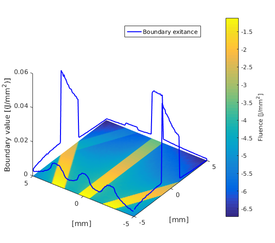
Plot the solution

hold on;

% The boundary solution is given as a constant fluence and extitance values
% at each boundary element.

% To plot the boundary fluence with plot3, an average coordinate of each
% boundary element is calculated


avgr = (vmcmesh.r(vmcmesh.BH(:, 1),:) + vmcmesh.r(vmcmesh.BH(:, 2),:))/2;
h = plot3(avgr(:,1), avgr(:,2), (solution.boundary_exitance), 'b','LineWidth',1.5);

% Draw the fluence in each element as before
patch('Faces', vmcmesh.H, 'Vertices',vmcmesh.r, 'FaceVertexCData', log(solution.element_fluence), 'FaceColor', 'flat', 'EdgeColor','none');
xlabel('[mm]');
ylabel('[mm]');
c = colorbar;                       % create a colorbar
c.Label.String = 'Fluence [J/mm^2]';
legend(h,{'Boundary exitance'});

% tilt the view
az = -54;
el = 34;
view([az, el]);
zlabel('Boundary value [(J/mm^2)]');

hold off