Simple example: simpletest.m

This example demonstrates how to setup a simple photon transport simulation, run it and visualise the result.

Contents

Create a triangular mesh

Function createRectangularMesh is used to setup a simple triangular mesh. The mesh is visualised in the figure below. Each element (a triangle) and boundary element (a line) in the mesh has a unique index that can be used to set their properties. The indices of the boundary elements are shown in the figure.

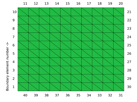
xsize =  10;	% width of the region [mm]
ysize =  10;	% height of the region [mm]
dh = 1;         % discretisation size [mm]
vmcmesh = createRectangularMesh(xsize, ysize, dh);

Give optical parameters

Constant optical parameters are set troughout the medium.

vmcmedium.absorption_coefficient = 0.01;     % absorption coefficient [1/mm]
vmcmedium.scattering_coefficient = 1.0;      % scattering coefficient [1/mm]
vmcmedium.scattering_anisotropy = 0.9;       % anisotropy parameter g of
                                             % the Heneye-Greenstein scattering
                                             % phase function [unitless]
vmcmedium.refractive_index = 1.3;            % refractive index [unitless]

Create a light source

Set up a 'cosinic' light source to boundary elements number 4,5,6 and 7. This means that the initial propagation direction with respect to the surface normal follows a cosine distribution. The photons are launched from random locations at these boundary elements.

vmcboundary.lightsource(4:7) = {'cosinic'};

% Run the Monte Carlo simulation
% Use the parameters that were generated to run the simulation in the mesh.
solution = ValoMC(vmcmesh, vmcmedium, vmcboundary);

                 ValoMC-2D
--------------------------------------------
  Version:  v1.0b-118-g853f111
  Revision: 131
  OpenMP enabled                     
  Using 16 threads
--------------------------------------------
Initializing MC2D...
Computing... 
...done

Done

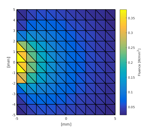
Plot the solution

The solution is given as an array in which the values represent a constant photon fluence in each element. This array can be plotted with Matlab's built-in function patch

patch('Faces',vmcmesh.H,'Vertices',vmcmesh.r,'FaceVertexCData', solution.element_fluence, 'FaceColor', 'flat', 'LineWidth',1.5);

hold on;

xlabel('[mm]');
ylabel('[mm]');
c = colorbar;                       % create a colorbar
c.Label.String = 'Fluence [W/mm^2]';
hold off

Published with MATLAB® R2016b