Directing light sources: directingls.m

This example demonstrates how to give custom directions to the light sources and how to use different built-in directivity patterns.

Set up the mesh and the medium
Set up the boundary and create light sources
Create and direct lightsources using different directivity patterns
Run the Monte Carlo simulation
Plot the solution

Set up the mesh and the medium

% Create a rectangular mesh
xsize =  10;    % width of the region [mm]
ysize =  10;    % width of the region [mm]
dh = 0.1;       % discretisation size [mm]
vmcmesh = createRectangularMesh(xsize, ysize, dh);

% Set constant background coefficients
vmcmedium.absorption_coefficient = 0.03;     % absorption coefficient [1/mm]
vmcmedium.scattering_coefficient = 0.3;      % scattering coefficient [1/mm]
vmcmedium.scattering_anisotropy = 0.9;       % scattering anisotropy parameter [unitless]
vmcmedium.refractive_index = 1.3;            % refractive index [unitless]

% Turn the fields in vmcmedium into arrays so that each coefficient can be
% set individually for each element
vmcmedium = createMedium(vmcmesh, vmcmedium);

rectangle_width = 1.9;
rectangle_height = 1.9;
rectangle_position=[-xsize/4 ysize/4];

% Find elements that are inside of a rectangle.
% The rectangle is shown in the figure below.
elements_of_the_rectangle = findElements(vmcmesh, 'rectangle', ...
                                         rectangle_position, ...
                                         rectangle_width, ...
                                         rectangle_height);

% Set the optical coefficients inside the rectangle
vmcmedium.absorption_coefficient(elements_of_the_rectangle) = 0.5;
vmcmedium.scattering_anisotropy(elements_of_the_rectangle) = 0.0;

Set up the boundary and create light sources

createBoundary returns a structure which can be used to set the properties of each boundary element individually

vmcboundary = createBoundary(vmcmesh);

Set up 4 lightsources using 4 lines. The lines are shown in the figure below.

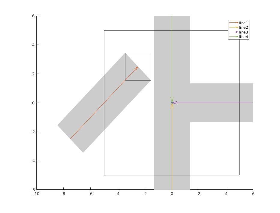
line1_start = [-3/4*xsize -ysize*1/4];
line1_end = rectangle_position;

rectangle_diameter = sqrt(rectangle_width^2+rectangle_height^2);
line_width=rectangle_diameter;

line2_start = [0 -3/5*ysize];
line2_end = [0 0];

line3_start = [3/5*xsize 0];
line3_end = [0 0];

line4_start = [0 3/5*ysize];
line4_end = [0 0];

lightsource1 = findBoundaries(vmcmesh, 'direction', ...
                              line1_start, ...
                              line1_end,  ...
                              line_width);

lightsource2 = findBoundaries(vmcmesh, 'direction', ...
                              line2_start, ...
                              line2_end,  ...
                              line_width);

lightsource3 = findBoundaries(vmcmesh, 'direction', ...
                              line3_start, ...
                              line3_end,  ...
                              line_width);

lightsource4 = findBoundaries(vmcmesh, 'direction', ...
                              line4_start, ...
                              line4_end,  ...
                              line_width);

Create and direct lightsources using different directivity patterns

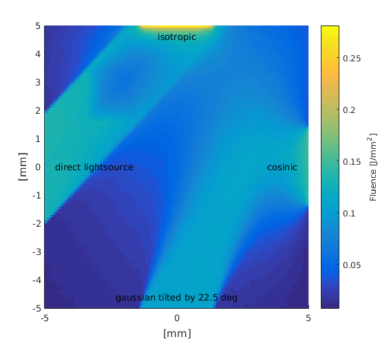
% 1: Direct light source
%
% The 'lightsource' -field in vmcboundary sets the directivity pattern of
% the lightsource. By 'direct' keyword, all photons are launched in the
% same direction.

vmcboundary.lightsource(lightsource1) = {'direct'};

% Create a direction vector for the light using the line that was used to
% search boundary elements
lightsource_direction = line1_end - line1_start;

% x-component of the direction
vmcboundary.lightsource_direction(lightsource1,1) = lightsource_direction(1);
% y-component of the dircetion
vmcboundary.lightsource_direction(lightsource1,2) = lightsource_direction(2);
% This means that the direction vector is given in the coordinate space of
% the mesh
vmcboundary.lightsource_direction_type(lightsource1) = {'absolute'};

% 2: A Gaussian light source
%
% Create a light source with a Gaussian directivity profile. The initial
% angles with respect to a given direction (by default, normal of the
% boundary element) follow a Gaussian with sigma = 0.1

vmcboundary.lightsource(lightsource2) = {'gaussian'};
vmcboundary.lightsource_gaussian_sigma(lightsource2) = 0.1;

% Tilt the lightsource by 22.5 degrees. This time, the direction is given in
% the coordinate system of the boundary element: (0, 1) is the normal
% direction and (1, 0) is directed along the boundary element
vmcboundary.lightsource_direction(lightsource2,1) = sin(-pi/8);
vmcboundary.lightsource_direction(lightsource2,2) = cos(-pi/8);

% this direction was given with respect to the surface normal
vmcboundary.lightsource_direction_type(lightsource2) = {'relative'};

% 3: Cosinic light source
%
% The initial angles follow a cosine distribution. Cosinic light sources
% are useful to create light sources that are not unidirectional without
% having to set any extra parameters.

vmcboundary.lightsource(lightsource3) = {'cosinic'};

% 4: Isotropic light source
%
% Photons are launched to all inward directions with an equal probability.

vmcboundary.lightsource(lightsource4) = {'isotropic'};

Run the Monte Carlo simulation

solution = ValoMC(vmcmesh, vmcmedium, vmcboundary);

                 ValoMC-2D
--------------------------------------------
  Version:  v1.0b-118-g853f111
  Revision: 131
  OpenMP enabled                     
  Using 16 threads
--------------------------------------------
Initializing MC2D...
Computing... 
...done

Done

Plot the solution