A photon transport simulation is initiated with

solution = ValoMC(mesh, medium, boundary, options);

solution = ValoMC(mesh, medium, boundary);

Documentation for each input structure and the output structure is provided here. Most of the fields in the input structures are arrays. For convenience, it is also possible to give the fields as scalars or as incomplete arrays. ValoMC will fill the arrays with the scalar value or complete them with the default values.

Input structures

1: mesh

The mesh structure defines the geometry of the problem.

Field name	Description	Unit	Element type [array size]
r	grid point coordinates	mm	double [N_r = number of coordinates in the system x 2]
H	indices to the grid points (triangles), i.e element topology	dimensionless	int64 [N_e = number of elements in the system x 3]
BH	indices to the boundary grid points (edges)	dimensionless	int64 [N_b = number of edges in the system x 2]
Optional fields
HN	neighborhood topology		int64 [N_e = number of elements in the system x 3]

Geometry description

A single area element is a triangle.

For example, a simple quadratic region that consists of two triangles can be built with the coordinate matrix

\begin{equation*} r = \left(\begin{array}{cc}-1 & -1\\-1 & 1\\1 & 1\\1 & -1\end{array}\right) \end{equation*}

and network topology matrices

\begin{equation*} H = \left(\begin{array}{ccc}1 & 2 & 3\\3 & 4 & 1\\\end{array}\right)\qquad\qquad\qquad\qquad BH = \left(\begin{array}{cc}1 & 2\\2 & 3\\3 & 4\\4 & 1\end{array}\right) \end{equation*}

The elements in H and BH refer to the rows in r. Each row in H refers to a single triangle and each row in BH refers to a single element boundary. As the quad has four edges and two triangles, there are four rows in BH and two rows in H. The matrices are illustrated in the figure below

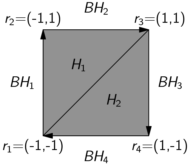
Note that the boundary lines are defined counterclockwise. While you can use clockwise or irregularly defined meshes, this might impair the functionality of 'findBoundaries' and make relative directions for lightsources ill defined.

2: medium

This structure is used to set the properties of the the medium. N_e is the number elements in the mesh. If a scalar value is given, it is applied to all elements.

Field name	Description	Unit	Element type [array size]
refractive_index	\(n\)	dimensionless	double [N_e] or [N_e x 2] (see below)
absorption_coefficient	\(\mu_a\)	1/mm	double [N_e] or [N_e x 2]
scattering_coefficient	\(\mu_s\)	1/mm	double [N_e] or [N_e x 2]
scattering_anisotropy	\(g\) (Henye-Greenstein phase function)	dimensionless	double [N_e] or [N_e x 2]

For detailed description of the coefficients, see e.g. the books by [Ihshimaru] and [Wang]

[Ishimaru] Wave Propagation and Scattering in Random Media, IEEE Press and Oxford University Press, 1997 [Wang] Biomedical Optics Principles and Imaging, Wiley, 2007

When two dimensional arrays are used, it is assumed that the mesh has been created with createGridMesh. The values then represent the values in each in grid point.

3: boundary

This structure is used to set the properties of the boundary surrounding the medium. N_b refers to the number of elements in the boundary. If a scalar value is given, it is applied to all elements.

Field name	Description	Unit	Element type [array size]
lightsource	Sets the light source type for each boundary element 'none': (default) no light source 'direct': direct light 'gaussian': the directivity follows a gaussian pattern (\(\sigma\) can be provided via optional fields) 'cosinic': the directivity follows a cosine pattern 'isotropic': photon packets will be launched at equal propability to all directions		double [N_b]
Optional fields
exterior_refractive_index	Sets the refractive index outside of the simulation geometry. This affects how the photon packets reflect when they encounter a boundary element.		double [N_b ]
Optional fields (lightsource)
lightsource_direction	Used to give a custom direction for a light source		double [N_b x 2 ]
lightsource_direction_type	Used to set the coordinate system in which the light direction is given 'relative': (default) light direction is given relative to the surface normal, i.e. (0,1) is the same as inward pointing surface normal and (1,0) is directed along the edge line. 'absolute': light direction is given in the position coordinate system		cell [N_b]
lightsource_irradiance	Sets the relative irradiance of the light source at each boundary element. (default=1)		double [N_b ]
Optional fields (lightsource='gaussian')
lightsource_gaussian_sigma	Standard deviation ( \(\sigma\) ) for a Gaussian light directivity pattern for each edge	radians	cell [N_b]

4: options

All fields are optional.

Field name	Description	Unit	Type
frequency	(default=0) Frequency of intensity modulation	1/s	double
phase0	(default=0) Phase at the lightsource for frequency modulation		double
seed	Random number generator seed (default={}) take seed from time		int64
photon_count	(default=1e6) Total number of photon packets		int64
disable_progressbar	(default=false) Set to true to disable progress bar		logical

Output structure

1: solution

Field name	Description	Unit	Element type [array size]
boundary_exitance	Exitance at each boundary element	W/mm2	double [N_b = number of boundary elements in the system ]
element_fluence	Fluence at each element	W/mm2	double [N_e = number of area elements in the system]
simulation_time	Total simulation time	seconds
Optional fields (options.seed=0)
seed_used	The random number seed that was used		double
Optional fields (multidimensional optical parameters)
grid_fluence	Fluence for two-dimensional optical parameters	W/mm2	double

Output description

The fluence is normalized so that that the integral of the exitance over the boundary 1 W when no photons are absorbed in the medium (i.e. \(\mu_a=0\)). This means the total power of a all light sources is in a single simulation is 1 W.