Working with Toast++: toastest.m

This example is based on a simple Toast++ usage example found on the Toast++ web site. The original example can be found from http://web4.cs.ucl.ac.uk/research/vis/toast/demo_matlab_fwd1.html. It simulates a steady state diffuse optical tomography (DOT) measurement in a circular geometry that has 16 detectors and 16 light sources located on the boundary of the object.

Each source is used to illuminate light into the domain and the amount of light is measured at all detectors. This is repeated for all source locations. In the example, the measurement matrix (signal intensity at each detector) is simulated both with Toast (as in the original example) and with ValoMC. Note that the results are not equal since Toast uses DA as the model for light propagation. DA can be regarded as a good approximation for photon transport in a highly scattering medium with distances further than a few scattering lengths from the source.

Toast++ is a software for image reconstruction in diffuse optical tomography. It contains a forward solver module using the finite element method for simulating the propagation of light in highly scattering, inhomogeneous biological tissues. The inverse solver module uses an iterative, regularized least-squares approach to reconstruct the unknown distributions of absorption and scattering coefficients in the volume of interest from boundary measurements of transmitted light.

Toast++ toolbox is being developed by Martin Schweiger and Simon Arridge (University College London) and the copyright of the original code belongs to them.

Toast homepage: http://web4.cs.ucl.ac.uk/research/vis/toast/index.html. M. Schweiger and S. R. Arridge, "The Toast++ software suite for forwards and inverse modeling in optical tomography", Journal of Biomedical Optics, 19(4):040801, 2014.

Create the geometry
Set the optical coefficients
Create the source and detector positions
Plot the source/detector arrangement
Solve the FEM system with Toast
Solve the photon transport problem with ValoMC
Plot the solutions
Plot the measurement profile as a function of source-detector separation

Create the geometry

Create a circular mesh using Toast++ and import it to ValoMC

rad = 25;
nsect = 8;
nring = 34;
nbnd = 2;


[vtx,idx,eltp] = mkcircle(rad,nsect,nring,nbnd);

toastmesh = toastMesh(vtx,idx,eltp);
vmcmesh = importToastMesh(toastmesh);

Set the optical coefficients

Note that the optical coefficients are given for each node in Toast, whereas in ValoMC they are uniform values for each element.

% absorption coefficient [1/mm]
mua_bkg = 0.01;
% scattering coefficient [1/mm]
mus_bkg = 1.0;
% scattering anisotropy parameter [unitless]
scattering_anisotropy_bkg = 0.0;
% reduced scattering coefficient [1/mm]
mus_reduced = mus_bkg*(1-scattering_anisotropy_bkg);

% Set optical coefficients for Toast.

nnd = toastmesh.NodeCount;
toast_mua = ones(nnd,1) * mua_bkg;  % absorption coefficient [1/mm]
toast_mus = ones(nnd,1) * mus_reduced; % reduced scattering coefficient [1/mm]

% Set optical coefficients for ValoMC. The refractive index is set but it
% does not affect the solution as there is no mismatch on the boundary.

nne = size(vmcmesh.H,1); % number of elements

% absorption coefficient [1/mm]
vmcmedium.absorption_coefficient = ones(nne,1)*mua_bkg;
 % scattering coefficient [1/mm]
vmcmedium.scattering_coefficient = ones(nne,1)*mus_bkg;
 % refractive index [unitless]
vmcmedium.refractive_index = ones(nne,1)*1;
% scattering anisotropy parameter [unitless]
vmcmedium.scattering_anisotropy = ones(nne,1)*scattering_anisotropy_bkg;

% Create the boundary so that there is no mismatch
vmcboundary = createBoundary(vmcmesh, vmcmedium);

Create the source and detector positions

A collimated lightsoure (pencil beam) can be approximated in DA by placing an isotropic source at a distance 1/mus' from the surface, where mus' is the reduced scattering coefficient.

% Build source/detector locations for Toast

nq = 16;
for ii=1:nq
  phi_q = 2*pi*(ii-1)/nq + pi / 256;
  Q(ii,:) = (rad - 1/mus_reduced) * [cos(phi_q) sin(phi_q)]; % source position
  phi_m = 2*pi*(ii-0.5)/nq + pi / 256;
  M(ii,:) = rad * [cos(phi_m) sin(phi_m)]; % detector position
end

toastmesh.SetQM(Q,M);


% Build source/detector locations for ValoMC

% Sources and detectors are placed to the nearest boundary elements

source_boundary_elements = findBoundaries(vmcmesh, 'location', Q);
detector_boundary_elements = findBoundaries(vmcmesh, 'location', M);

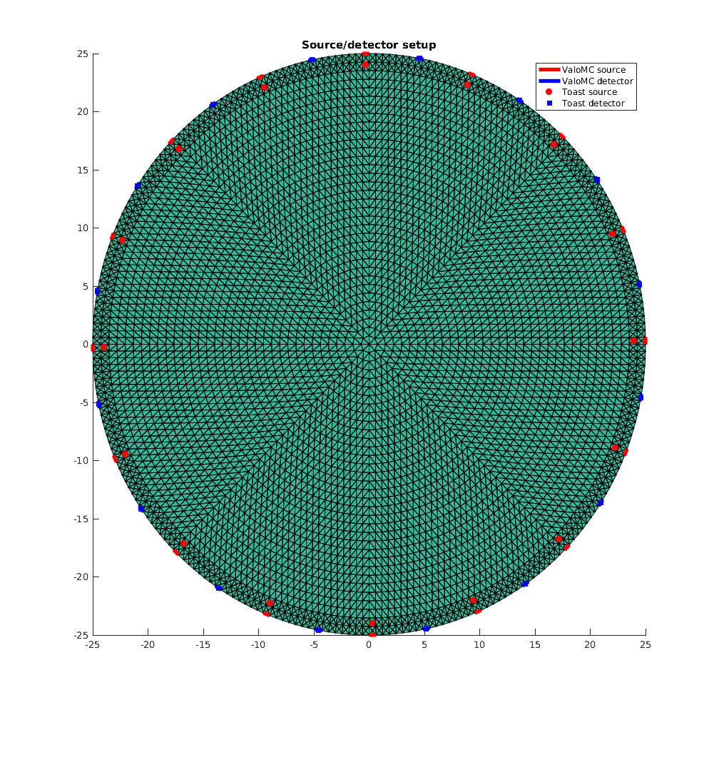
Plot the source/detector arrangement

Note that the lightsources have a finite width in ValoMC, which introduces a small discretisation error in the comparison.

figure('rend','painters','pos',[10 10 1000 1000])
hold on
patch('Faces', vmcmesh.H, 'Vertices',vmcmesh.r, 'FaceVertexCData', 0, 'FaceColor', 'flat', 'LineWidth', 0.1);

for ii=1:nq
    h1=plot(vmcmesh.r(vmcmesh.BH(source_boundary_elements(ii),:),1), ...
            vmcmesh.r(vmcmesh.BH(source_boundary_elements(ii),:),2), 'r', 'LineWidth',4.0);
    h2=plot(vmcmesh.r(vmcmesh.BH(detector_boundary_elements(ii),:),1), ...
            vmcmesh.r(vmcmesh.BH(detector_boundary_elements(ii),:),2), 'b', 'LineWidth',4.0);
end

h3 = plot(Q(:, 1),Q(:,2),'ro','MarkerFaceColor','r');
h4 = plot(M(:, 1),M(:,2),'bs','MarkerFaceColor','b');

title('Source/detector setup');
legend([h1 h2 h3 h4], {'ValoMC source', 'ValoMC detector', 'Toast source', 'Toast detector'});
hold off

Solve the FEM system with Toast

The system matrix is constructed manually using 2D coefficients (by default, Toast uses formulas derived from the radiative transfer equation for 3D geometry). For more detailed information about 2D and 3D coefficients, see e.g. T. Tarvainen: Computational Methods for Light Transport in Optical Tomography, PhD thesis, University of Kuopio, 2006.

% Create isotropic sources
qvec = toastmesh.Qvec('Isotropic','Point');

% To obtain comparable results, the measurement vectors have a sharp
% Gaussian profile (a narrow detector). Conversion factor between fluence
% and exitance is 2/pi in 2D
mvec = 2/pi*toastmesh.Mvec('Gaussian',0.5,0);

% 2D diffusion coefficient
toast_kap = 1./(2.*(toast_mua+toast_mus));

S1 = toastmesh.SysmatComponent('PFF',toast_mua);
S2 = toastmesh.SysmatComponent('PDD',toast_kap);

% The boundary term is multiplied by 2/pi in 2D
S3 = toastmesh.SysmatComponent ('BndPFF', ones(nnd,1)*2/pi);
K = S1+S2+S3;

Phi = K\(qvec);                % solve the fluence
Y_toast  = mvec.' * Phi;       % compute the exitance on each detector

Solve the photon transport problem with ValoMC

The source is relocated 16 times and the exitance at each 16 detector is stored to build a similar source/detector matrix as in the original example.

Y_vmc = ones(nq,nq);
for ii=1:16
   disp(['Starting simulation ' num2str(ii) ' out of ' num2str(nq)]);
   options.photon_count = 1e8;            % number of photon packets
   vmcboundary.lightsource(:) = {'none'}; % erase all previous light sources
   % use a collimated light source
   vmcboundary.lightsource(source_boundary_elements(ii)) = {'direct'};
   vmcsolution = ValoMC(vmcmesh, vmcmedium, vmcboundary, options);
   % build the solution matrix column by column
   Y_vmc(:,ii) = vmcsolution.boundary_exitance(detector_boundary_elements(:));
end

Starting simulation 1 out of 16
                 ValoMC-2D
--------------------------------------------
  Version:  v1.0b-118-g853f111
  Revision: 131
  OpenMP enabled                     
  Using 16 threads
--------------------------------------------
Initializing MC2D...
Computing... 
...done

Done
Starting simulation 2 out of 16
                 ValoMC-2D
--------------------------------------------
  Version:  v1.0b-118-g853f111
  Revision: 131
  OpenMP enabled                     
  Using 16 threads
--------------------------------------------
Initializing MC2D...
Computing... 
...done

Done
Starting simulation 3 out of 16
                 ValoMC-2D
--------------------------------------------
  Version:  v1.0b-118-g853f111
  Revision: 131
  OpenMP enabled                     
  Using 16 threads
--------------------------------------------
Initializing MC2D...
Computing... 
...done

Done
Starting simulation 4 out of 16
                 ValoMC-2D
--------------------------------------------
  Version:  v1.0b-118-g853f111
  Revision: 131
  OpenMP enabled                     
  Using 16 threads
--------------------------------------------
Initializing MC2D...
Computing... 
...done

Done
Starting simulation 5 out of 16
                 ValoMC-2D
--------------------------------------------
  Version:  v1.0b-118-g853f111
  Revision: 131
  OpenMP enabled                     
  Using 16 threads
--------------------------------------------
Initializing MC2D...
Computing... 
...done

Done
Starting simulation 6 out of 16
                 ValoMC-2D
--------------------------------------------
  Version:  v1.0b-118-g853f111
  Revision: 131
  OpenMP enabled                     
  Using 16 threads
--------------------------------------------
Initializing MC2D...
Computing... 
...done

Done
Starting simulation 7 out of 16
                 ValoMC-2D
--------------------------------------------
  Version:  v1.0b-118-g853f111
  Revision: 131
  OpenMP enabled                     
  Using 16 threads
--------------------------------------------
Initializing MC2D...
Computing... 
...done

Done
Starting simulation 8 out of 16
                 ValoMC-2D
--------------------------------------------
  Version:  v1.0b-118-g853f111
  Revision: 131
  OpenMP enabled                     
  Using 16 threads
--------------------------------------------
Initializing MC2D...
Computing... 
...done

Done
Starting simulation 9 out of 16
                 ValoMC-2D
--------------------------------------------
  Version:  v1.0b-118-g853f111
  Revision: 131
  OpenMP enabled                     
  Using 16 threads
--------------------------------------------
Initializing MC2D...
Computing... 
...done

Done
Starting simulation 10 out of 16
                 ValoMC-2D
--------------------------------------------
  Version:  v1.0b-118-g853f111
  Revision: 131
  OpenMP enabled                     
  Using 16 threads
--------------------------------------------
Initializing MC2D...
Computing... 
...done

Done
Starting simulation 11 out of 16
                 ValoMC-2D
--------------------------------------------
  Version:  v1.0b-118-g853f111
  Revision: 131
  OpenMP enabled                     
  Using 16 threads
--------------------------------------------
Initializing MC2D...
Computing... 
...done

Done
Starting simulation 12 out of 16
                 ValoMC-2D
--------------------------------------------
  Version:  v1.0b-118-g853f111
  Revision: 131
  OpenMP enabled                     
  Using 16 threads
--------------------------------------------
Initializing MC2D...
Computing... 
...done

Done
Starting simulation 13 out of 16
                 ValoMC-2D
--------------------------------------------
  Version:  v1.0b-118-g853f111
  Revision: 131
  OpenMP enabled                     
  Using 16 threads
--------------------------------------------
Initializing MC2D...
Computing... 
...done

Done
Starting simulation 14 out of 16
                 ValoMC-2D
--------------------------------------------
  Version:  v1.0b-118-g853f111
  Revision: 131
  OpenMP enabled                     
  Using 16 threads
--------------------------------------------
Initializing MC2D...
Computing... 
...done

Done
Starting simulation 15 out of 16
                 ValoMC-2D
--------------------------------------------
  Version:  v1.0b-118-g853f111
  Revision: 131
  OpenMP enabled                     
  Using 16 threads
--------------------------------------------
Initializing MC2D...
Computing... 
...done

Done
Starting simulation 16 out of 16
                 ValoMC-2D
--------------------------------------------
  Version:  v1.0b-118-g853f111
  Revision: 131
  OpenMP enabled                     
  Using 16 threads
--------------------------------------------
Initializing MC2D...
Computing... 
...done

Done

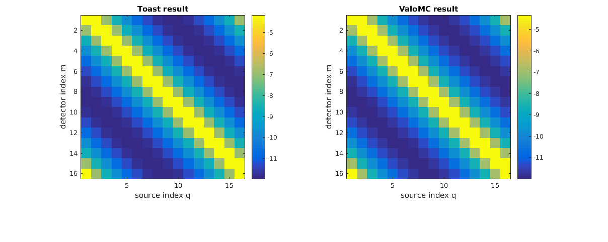
Plot the solutions

figure('rend','painters','pos',[10 10 1200 400])

subplot(1,2,1)
imagesc(log(Y_toast));
xlabel('source index q');
ylabel('detector index m');
axis equal tight;
colorbar
title('Toast result');

% Display boundary profile

subplot(1,2,2)
imagesc(log(Y_vmc));
xlabel('source index q');
ylabel('detector index m');
axis equal tight;
colorbar
title('ValoMC result');
hold off;

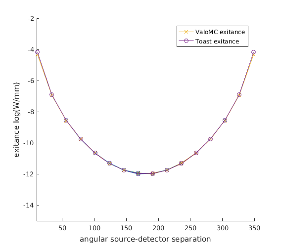
Plot the measurement profile as a function of source-detector separation

Note that because of the differences between the diffusion approximation and radiative transport theory, discretization errors as well as the stochastic nature of the Monte Carlo simulations, the 16 measurement profiles do not fully coincide.

figure
hold on

angle = 360/32:360/16:360;

for profile_number=1:16

   h1=plot(angle, log(circshift((Y_vmc(:,profile_number)),-(profile_number-1))),'x-');
   h2=plot(angle, log(circshift((Y_toast(:,profile_number)),-(profile_number-1))),'o-');

   axis([10 350 -15 -2]);
   xlabel('angular source-detector separation');
   ylabel('exitance log(W/mm)');

end

legend([h1 h2], {'ValoMC exitance', 'Toast exitance'});


hold off