Simulating the photoacoustic effect using k-Wave: kwavetest.m

This example demonstrates simulation of a pressure field generated through the absorption of an externally introduced light pulse. The light propagation is simulated using ValoMC and the propagation and detection of pressure wavefield is simulated using k-Wave, see http://www.k-wave.org/documentation/k-wave_initial_value_problems.php. The example also shows how the computation grid of k-Wave and mesh of ValoMC can be made compatible. Note that k-Wave uses SI units (e.g. [m]) and ValoMC works in millimetre-scale (e.g. [mm]).

k-Wave is an open source acoustics toolbox for MATLAB and C++ developed by Bradley Treeby and Ben Cox (University College London) and Jiri Jaros (Brno University of Technology). The software is designed for time domain acoustic and ultrasound simulations in complex and tissue-realistic media.

k-Wave homepage: http://www.k-wave.org/. B. E. Treeby and B. T. Cox: "k-Wave: MATLAB toolbox for the simulation and reconstruction of photoacoustic wave-fields", Journal of Biomedical Optics, 15(2):021314, 2010.

Note: there was an incorrectly explained unit conversion earlier in this example. See the text shown in red.

Contents

k-Wave initialisation

The initialisation is done as normal in k-Wave. Care must be taken at the initialization ValoMC, to make a matching computational simulation area for (see ValoMC initialization) the photon propagation simulation.

clear all;

% Create the k-Wave grid
Nx = 150;           % number of grid points in the x (row) direction
Ny = 150;           % number of grid points in the y (column) direction
dx = 0.1e-3;        % grid point spacing in the x direction [m]
dy = 0.1e-3;        % grid point spacing in the y direction [m]
kgrid = makeGrid(Nx, dx, Ny, dy);

% Create two internal structures using makeDisk
discs = makeDisc(Nx, Ny, 55, 55, 5) + makeDisc(Nx, Ny, 75, 85, 10);


% Define the acoustic properties
disc_indices = find(discs==1);

medium.sound_speed = 1500*ones(Nx, Ny);    % [m/s]
medium.sound_speed(disc_indices) = 1800;   % [m/s]

medium.density = 1000*ones(Nx, Ny);        % [kg/m^3]
medium.density(:,Ny/2:end) = 1400;

WARNING: makeGrid will be deprecated in a future version of k-Wave.
         Update codes to use the syntax kgrid = kWaveGrid(...).

Create a ValoMC mesh

ValoMC uses triangles and tetrahedrons as the basis shape, whereas in k-Wave pixels and voxels are used. createGridMesh can be used to create a straightforward mapping between the triangles and pixels. Note that K-Wave uses matrices in the format matrix(X,Y), whereas MATLAB t(c.f. meshgrid) and ValoMC uses matrix(Y,X) Therefore x and y should be swapped when moving between ValoMC arrays and k-Wave arrays

vmcmesh = createGridMesh(kgrid.y_vec*1e3, kgrid.x_vec*1e3); % [m to mm]

Define optical coefficients

For users accustomed to k-Wave, the optical coefficients can be set in similar fashion as in k-Wave, i.e. using multidimensional arrays. If one of the arrays defining the medium is given as multidimensional array to ValoMC, the code will assume that the mesh was created using 'createGridMesh' and the output fluence will also given as a two dimensional array in solution.grid_fluence. See the example 'Working with pixel and voxel data' on how to achieve similar assignments using one dimensional indexing.

vmcmedium.scattering_coefficient = 0.01*ones(Nx, Ny);
vmcmedium.absorption_coefficient = 0.001*ones(Nx, Ny);
discs = makeDisc(Nx, Ny, 55, 55, 5) + makeDisc(Nx, Ny, 75, 85, 10);
% Define the acoustic properties
disc_indices = find(discs==1);

vmcmedium.absorption_coefficient(disc_indices) = 0.01;
vmcmedium.scattering_anisotropy = 0.9;           % scattering anisotropy parameter [unitless]
vmcmedium.refractive_index = 1.0*ones(Nx, Ny);
vmcmedium.refractive_index(:,Ny/2:end) = 1.4;    % refractive index [unitless]

% Define the Gruneisen parameter describing photoacoustic efficiency
vmcmedium.gruneisen_parameter = 0.02*ones(Nx, Ny);      % [unitless]

Create a light source

% Set a light source with a width of 2 mm and cosinic directional profile
% in -x direction
boundary_with_lightsource = findBoundaries(vmcmesh, 'direction', ...
                                           [0 0], ...
                                           [-10 0], ...
                                           2);

vmcboundary.lightsource(boundary_with_lightsource) = {'cosinic'};

Run the Monte Carlo simulation

solution = ValoMC(vmcmesh, vmcmedium, vmcboundary);

                 ValoMC-2D
--------------------------------------------
  Version:  v1.0b-118-g853f111
  Revision: 131
  OpenMP enabled                     
  Using 16 threads
--------------------------------------------
Initializing MC2D...
Computing... 
...done

Done

Compute the initial pressure from the photon fluence

Note that since the medium was defined as two dimensional arrays, the output is also given as a two-dimensional array.

Corrected explanation

% Compute the absorbed optical energy density.
% multiply by
% 1e6   to convert [J/mm^2] to [J/m^2]
% 1e-3  to set the total energy in the pulse to 1 mJ
%
vmcmedium.absorbed_energy = vmcmedium.absorption_coefficient .* solution.grid_fluence*1e3; % [J/m3]

% Compute the initial pressure distribution
source.p0 = vmcmedium.gruneisen_parameter .* vmcmedium.absorbed_energy;  % [Pa]

Define the k-Wave sensor mask

% Define a circular sensor
sensor_radius = 4e-3;       % [m]
num_sensor_points = 50;     % number of sensor points

sensor.mask = makeCartCircle(sensor_radius, num_sensor_points);

Move the perfectly matched layer (PML) outside of the computation domain and run the acoustic simulation

The PML is a layer that absorbs waves for simulating free regions and is normally contained within the computation region of k-Wave. For a more straightforward mapping between the computation region of k-Wave and ValoMC, the PML is moved outside of the computation region.

sensor_data = kspaceFirstOrder2D(kgrid, medium, source, sensor, 'PMLInside', false);

Running k-Wave simulation...
  start time: 11-Feb-2020 17:43:38
  reference sound speed: 1800m/s
  WARNING: visualisation plot scale may not be optimal for given source.
  dt: 16.6667ns, t_end: 14.1333us, time steps: 849
  input grid size: 150 by 150 grid points (15 by 15mm)
  maximum supported frequency: 7.5MHz
  smoothing p0 distribution...
  expanding computational grid...
  computational grid size: 190 by 190 grid points
  WARNING: Highest prime factors in each dimension are 19  19
           Use dimension sizes with lower prime factors to improve speed
  calculating Delaunay triangulation...
  precomputation completed in 0.6779s
  starting time loop...
  estimated simulation time 8.6441s...
  simulation completed in 8.3875s
  total computation time 9.1863s

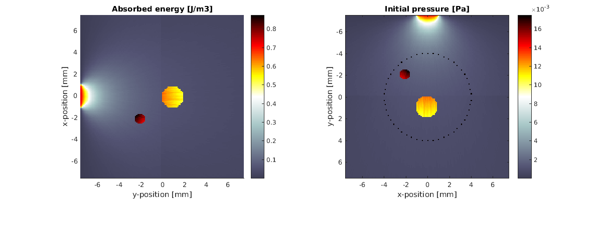
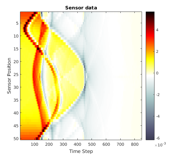
Plot the solution

figure('rend','painters','pos',[10 10 1200 400])

% plot the initial pressure and sensor distribution
subplot(1,2,1)
hold on

% We have to swap x and y again
imagesc(kgrid.y_vec*1e3, kgrid.x_vec*1e3, vmcmedium.absorbed_energy, [min(vmcmedium.absorbed_energy(:)) ...
        max(vmcmedium.absorbed_energy(:))]);

xlabel('y-position [mm]');
ylabel('x-position [mm]');
colormap default;

c = colorbar;  % create a colorbar
axis image;
title('Absorbed energy [J/m3]');
hold off

subplot(1,2,2)

imagesc(kgrid.x_vec*1e3, kgrid.y_vec*1e3, transpose(source.p0 + ...
        cart2grid(kgrid, sensor.mask)), [min(source.p0(:)) ...
        max(source.p0(:))]);


colormap(getColorMap);
xlabel('x-position [mm]');
ylabel('y-position [mm]');
c = colorbar;  % create a colorbar
axis image;
title('Initial pressure [Pa]');
hold off

% plot the simulated sensor data
figure;
imagesc(sensor_data,  [min(sensor_data(:)) max(sensor_data(:))]);
colormap(getColorMap);
ylabel('Sensor Position');
xlabel('Time Step');
c = colorbar;  % create a colorbar
colorbar;
title('Sensor data');

Published with MATLAB® R2016b