Netgen 3D example

This example demonstrates how to setup a 3D simulation on a geometry built with Netgen and run it. The geometry is a sphere within a cube. The sphere has a different refractive index than the cube. The mesh is created so that there is a circular domain within one surface of the cube. You can view the Netgen Python source code here

Note: This is example requires a powerful computer to run.

Import the NetGen file
Find indices from the file
Set optical coefficients
Find boundary elements
Plot the mesh
Run the simulation
Visualize the solution

Import the NetGen file

clear all;

if(exist('sphere_in_box.vol', 'file') ~= 2)
    error('Could not find the mesh data file. Please run netgen netgen_sphere_in_box.py');
end

[vmcmesh regions region_names boundaries boundary_names] = importNetGenMesh('sphere_in_box.vol', false);

Find indices from the file

background = cell2mat(regions(find(strcmp(region_names,'background'))));
sphere = cell2mat(regions(find(strcmp(region_names,'sphere'))));

Set optical coefficients

vmcmedium.absorption_coefficient(:) = 0.01;
vmcmedium.scattering_coefficient(:) = 0.01;
vmcmedium.scattering_anisotropy(:) = 0.9;
vmcmedium.refractive_index(:) = 1.0;

% Use the indices
vmcmedium.absorption_coefficient(background) = 0.01;
vmcmedium.scattering_coefficient(background) = 0.3;
vmcmedium.scattering_anisotropy(background) = 0.9;
vmcmedium.refractive_index(background) = 1.0;

vmcmedium.absorption_coefficient(sphere) = 0.01;
vmcmedium.scattering_coefficient(sphere) = 0.3;
vmcmedium.scattering_anisotropy(sphere) = 0.9;
vmcmedium.refractive_index(sphere) = 1.7;

Find boundary elements

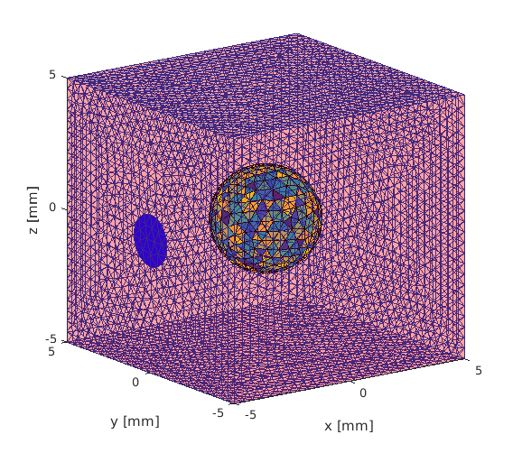
A circular domain for the light source was meshed (circle r = 1.0 at the face of the cube whose normal points to [-1 0 0]) but it is not contained as a separate boundary condition. We can use findBoundaries to find it manually.

lightsource1 = findBoundaries(vmcmesh, 'direction', [0 0 0 ], [-5 0 0], 1.1);
vmcboundary.lightsource(lightsource1) = {'direct'};

Plot the mesh

figure
hold on

trimesh(vmcmesh.BH,vmcmesh.r(:,1),vmcmesh.r(:,2),vmcmesh.r(:,3),'facecolor', 'r','FaceAlpha',0.2);

% Highlight the location for the lightsource for the plot
trimesh(vmcmesh.BH(lightsource1,:),vmcmesh.r(:,1), vmcmesh.r(:,2),vmcmesh.r(:,3),'facecolor', 'b');
% Show the sphere
tetramesh(vmcmesh.H(sphere,:), vmcmesh.r);

xlabel('x [mm]');
ylabel('y [mm]');
zlabel('z [mm]');
view(-36,16);

hold off

Run the simulation

options.photon_count=1e8;
solution = ValoMC(vmcmesh, vmcmedium, vmcboundary,options);

                 ValoMC-3D
--------------------------------------------
  Version:  v1.0b-118-g853f111
  Revision: 131
  OpenMP enabled                     
  Using 16 threads
--------------------------------------------
Initializing MC3D...
Computing... 
...done

Done

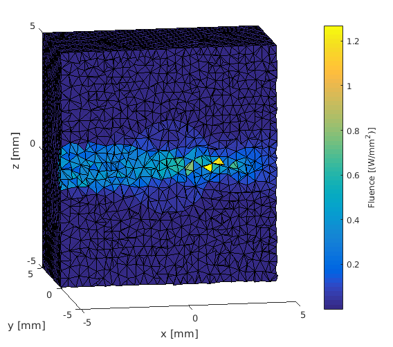
Visualize the solution

Visualizing large tetrahedral meshes is often cumbersome. Alternative, less power consuming option is to use exportX3D to export solution to X3D format and view the file using e.g. meshlab. See 'help exportX3D' for more details.

figure
hold on
halfspace_elements = findElements(vmcmesh, 'halfspace', [0 0 0], [0 1 0]);
tetramesh(vmcmesh.H(halfspace_elements,:), vmcmesh.r, solution.element_fluence(halfspace_elements));
view(-10,10);
%
%hold
xlabel('x [mm]');
ylabel('y [mm]');
zlabel('z [mm]');

c = colorbar;
c.Label.String = 'Fluence [(W/mm^2)]';